One way to do stochastic halftoning is to draw contours of noise functions. For example, you can make 2D single-frequency Fourier noise, and draw a contour wherever the noise crosses the zero-level. If you do this with wavelength L, over an area of A, the total arc length turns out to be very nearly 2.2*A/L. Why? And what’s the exact value? Time to dive into probability.
Let’s define the noise field as a sum of N randomly tilted sinusoids:
\begin{aligned}h=\sum_i^N \cos \left( 2 \pi \left( x \cos(t_i)-y \sin(t_i) +p_i \right)/L \right) \end{aligned},
where t_i, p_i are random angles, and x,y are spatial positions.
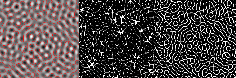
Its probability density function is f_h, and cumulative density function is F_h. With that, we could find the relative area of the noise field that is within some small absolute value around zero: F_h(h\geq \epsilon) - F_h(h\geq -\epsilon). You can think of this as a band of space around the zero-contour, with varying width. Ideally, we would find some transformed noise field, r, where that band has a uniform width, then divide its area by its width to find the arc length, s. You can see an example of these bands in the image above.
The easy way to do that is to scale h by its gradient, enforcing a unit gradient at the zero-crossing. That is, r=h/|\nabla h|. With that, we know that the band within \pm \epsilon of zero has width 2 \epsilon, so the arc length is roughly (F_r(r\geq \epsilon) - F_r(r\geq -\epsilon))/(2 \epsilon). This is of course a derivative, so as \epsilon \rightarrow 0, it becomes s=f_r(r=0).
Now all we need to do is find f_r(r=0). To start, let’s define the transformed noise:
\begin{aligned} r &= \frac{h}{g} \\ g &= \sqrt{g_x^2+g_y^2} \\ g_x &= \frac{d h}{dx} \\ g_y &= \frac{d h}{dy} \end{aligned}.
Keeping track of all the original variables t_i, p_i,x,y is a hassle. Instead, we can say that p_i takes care of all of the phase in h. Then we get:
\begin{aligned} h &= \sum_i^N \cos (p_i) \\ g_x &= \sum_i^N \frac{-2\pi }{L}\cos(t_i) \sin(p_i) \\ g_y &= \sum_i^N \frac{2\pi }{L}\sin(t_i) \sin(p_i)\end{aligned}.
With these, it’s time for a couple big assumptions. I’ll say that h,g_x, g_y are all independent. This isn’t strictly true, but the dependence is very weak due to the summation of many sinusoids. It also makes the math so much easier!
Now it’s time to build up some pdfs. The variance of a single component sinusoid is \sigma_{h_1}^2=1/2, and if we add together many, we can take advantage of the Central Limit Theorem (CLT). This tells us that the total should be normally distributed with \sigma_{h}=\sigma_{h_1} \sqrt{N} = \sqrt{N/2}. So with large N, we get
f_h = \frac{1}{\sqrt{N \pi}} \exp \left( \frac{-x^2}{n} \right) .
That one was easy. Time to build g_x. For a single sinusoid, \sigma_{g_{x1}}^2=\pi^2/L^2. Again with the CLT, we get \sigma_{g_x} = \pi\sqrt{N}/L. Then we have
f_{g_x} = \frac{L}{\pi^{3/2}\sqrt{2N}} \exp \left( \frac{-x^2 L^2}{2N \pi^2} \right).
Now we transform that to find f_{g_x^2}:
\begin{aligned}f_{g_x^2} &= \frac{f_{g_x}(x=\sqrt{y})}{ 2 \sqrt{y} }+\frac{f_{g_x}(x=-\sqrt{y})}{ 2 \sqrt{y} } \\ &= \frac{L}{\pi^{3/2} \sqrt{2 N y}} \exp \left( \frac{-y^2 L^2}{2 N \pi^2} \right) . \end{aligned}
To get to g_x^2+g_y^2, the easy way is to recognize f_{g_x^2} as a gamma distribution, and know that the sum of two gamma distributions is itself a gamma distribution. That lets us write
f_{g_x^2+g_y^2} = \frac{L^2}{2 N\pi^2} \exp \left( \frac{-y L^2}{2 N \pi^2} \right) .
Now the square-root to find f_g:
\begin{aligned}f_g &= \frac{f_{g_x^2+g_y^2}(y=z^2)}{ 1/(2 z) } \\ &= \frac{z L^2}{ N\pi^2} \exp \left( \frac{-z^2 L^2}{2 N \pi^2} \right) . \end{aligned}
Finally, we get to f_r. First, define v=g, \, w=r=h/g, then find the determinant of this transformation, which turns out to be v, and so
\begin{aligned}f_{r} &= \int_0^\infty v f_h f_g dv\\ &= \frac{\pi L^2}{\sqrt{2} \left(2 \pi^2 w^2 + L^2 \right)^{3/2}} . \end{aligned}
Finally! The curve length per unit area is thus f_r(w=0)=\pi/(L \sqrt{2}) \approx 2.22144/L. My curiosity is satisfied.
And now I can use it for halftoning! Check out the result on a skull:
