Time for some competing acronyms. Fluids people like to call this technique Proper Orthogonal Decomposition (POD), statisticians call it Principal Component Analysis (PCA), and so on and so on. Whatever you want to call it, it’s basically an eigenvector decomposition of the data you toss into it. That means that it optimally splits the data along a set of orthogonal axes, and orders them so that the first set contains the most `energy’ in the data, and decreases from there.
That’s a bit abstract, so let’s apply it to the PIV data of a cylinder:

If we apply POD to this data, it will give a set of spatial modes and time amplitudes that describe the behavior of the flow. Ideally, a small number of these modes will accurately represent the flow.
How does POD work? Eigenvalues, basically. Read on for the math, or jump further down the page to skip it.
Math ahead:
Now for some math, just to be rigorous, using nomenclature from Dudok de Wit et al. Assume that the data, y, is captured over M spatial points (x) and N time points (t), over N instants. The data set is arranged into the matrix Y , where each column consists of the data from a single instant in time. A singular value decomposition is used to extract the spatial eigenmodes \phi_k ( k^{th} column of \phi ), temporal eigenmodes \psi_k ( k^{th} column of \psi ), and weights A_k (along the diagonal of A ). The spatial and temporal eigenmodes are independently orthogonal. The number of modes is the smaller of M or N. The behavior of a single mode can be extracted as Y_k .
Y_{i,j} = y(x_j,t_i) = \sum_{k=1}^{N} A_k \phi_k(x_j) \psi_k(t_i)
Y = \phi A \psi^T
Y_k = \phi_k A_k \psi_k^T
\sum \psi_k \psi_l = \sum \phi_k \phi_l = \delta_{kl}
In MATLAB, the singular value decomposition is computed with the command svd. Each eigenmode has a norm of 1, and they are sorted by the weights x A_k in decreasing order. In the case of velocity measurements, the weights are proportional to the kinetic energy of the flow.
\left[\phi, A, \psi \right] = \text{svd}\left(Y\right)
||\psi_k|| = 1
||\phi_k|| = 1
||Y_k|| = A_k
An alternative means of computation is the method of snapshots. To save memory and computation, the svd (Y) is not computed directly. Instead, (\phi,\Sigma, \psi) are computed as below. After ensuring that the eigenvalues are sorted in descending order, \phi is computed, and the analysis proceeds as before. The method of snapshots is appropriate to use when the number of measurement points greatly exceeds the number of observations. This is quite common in simulations of fluids, or with PIV data.
\left[ \psi, A^2 \right] = \text{eig}(Y^T Y )
\phi = Y \psi A^{-1}
You have survived the Math.
Looking at POD Results
Practically, how should we apply POD? Generally, the mean should be subtracted before running POD. This basically reduces the workload of POD, and mathematically encourages it to look at other variation in the data. So let’s thow the (temporal) mean-subtracted data into POD. We get three things: Singular values, mode shapes, and time-amplitudes. First, let’s look at the distribution of singular values:

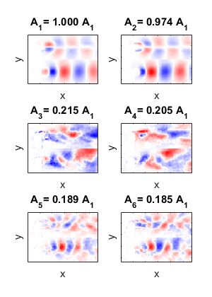
The first two modes are the most energetic, by far. Beyond that, the energy spectrum tapers off. What do those first two modes look like? Here are the first six mode shapes:

These are titled by the relative amplitudes of their singular values. You can see that they appear to be paired in shape and amplitude, and look like traveling waves. Modes #1 and #2 contain the large-scale flapping, and #5 and #6 look like the half-wavelength oscillations. The middle pair are less clear, but deal with some sort of asymmetry. How do these modes vary in time? Here are the time-amplitudes of those modes:

These amplitudes make some sense, with respect to the modes. Regular oscillations from the first pair (though a quarter-cycle out of phase), higher-frequency oscillations from the third pair, and weirdness from the second pair.
One of the nice things about POD is that you can try to make a smaller (and cleaner) version of the data. Since the POD modes are ordered by their coherence and energy, the low-ranked POD modes often represent noise in the data, and can be removed to make things look better. For example, here are a few reconstructions using 6, 20, and 100 (out of 100) modes:

You can see that the reconstruction with 6 modes captures the general behavior quite well, but loses the small details. Reconstruction with 100 modes is identical to the original data, and 20 modes is somewhere in the middle.
If you’d like to play with the data or code, here it is.
Some Advice
- POD applied to velocity data sorts the modes by their kinetic energy. If you apply it to vorticity, it’ll sort by enstrophy. If you mix velocity data with another type of data, such as force measurements, you can no longer reliably talk about physical energy. POD will still extract the dominant modes, but different scalings on the voltage vs velocity will result in different results.
- POD modes are not guaranteed to contain the dynamics of the system. You may want to make a low-order model with the first few modes, but it may not work at all.
- This applied POD in the temporal domain, but the data set could also be sliced spatially, where the axes of each frame are time and space. This analysis would then other potentially interesting results. This could work well if one spatial dimension is time-like, as in convecting flows.
- The different frames don’t need to be equally spaced in time to apply POD. With the extracted time-amplitudes, you can interpolate to get an estimated data set at a given rate.
- Since the time-amplitudes are all orthogonal, you can use them as basis functions for decomposing other data. This is the basis of Extended POD.