I wanted to try some different grid-based dithering methods, so here we go: quadtree subdivisions, dither matrices, dithering along space-filling curves, and a hill-climbing optimization.
Quadtree Dithering
This uses recursive subdivision to distribute blackness in the image. The general idea is to make sure that each subdivision contains an integer number of black dots, and refine until a subdivision has zero or one dots. If it has one dot, draw it. To begin with, ensure that the total blackness of the image is an integer, and the image is square with 2^k pixels per side. Then treat the image as the first subdivision:
- Calculate the total blackness in the region, K, which is equal to the number of dots within, N.
- Split the square image into quadrants.
- For each quadrant, compute the blackness within K_i. This is not necessarily an integer, so make an initial estimate of N_i = \text{floor}(K_i).
- We want \sum N_i = N. If \sum N_i \neq N:
- Define n = \sum N_i - N. For the n subdivisions with the largest K_i-N_i, increase N_i by one.
- For each subdivision, multiply the interior pixel values by N_i/K_i. This ensures an integer total within.
- For subdivisions with N_i=1, place a dot. If N_i > 1, divide it into quadrants and return to step 1 for each quadrant.

This works, but doesn’t look great. Oh well!
Dither Matrices
A dither matrix is compared directly to the image: any darker pixels are retained, and lighter ones are discarded. So what’s a good way to make a dither matrix? Generally, each additional dot should be far from other points, and should avoid making recognizable patterns.
Here are a few of my attempts. I used a matrix of 20×20 pixels, and I used toroidal distance. That is, I computed the x-distance as min(|x_2-x_1|, n_x/2) , where n_x is the width of the matrix.
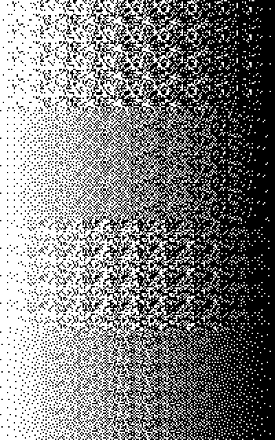
First attempt: a random matrix. I randomly distributed the integers from 0 to 199 on the matrix, and scaled them to be in the image range of 0-1. This is the top section of the image above. This gives the right tone on average, but it has weird clumps.
Second attempt: picking the farthest point, and saving the order. When I started with this, it created very regular patterns. I learned that you have to include some randomness to avoid checkerboards and the like. In the image above, this is the second section. At left, the first points are still pretty regularly distributed, but generally looks OK. Unfortunately, the dark end is a bit clumpy, as these were the last points available to be chosen.
Third attempt: reusing the previous results and separating even/odd. My idea was that if the even points are kept at the light end, and the odd points are moved to the dark end, this should improve the behavior in very light and very dark areas. The result is the third section of the image. This alteration did make the point distribution more symmetric at the light and dark ends, but introduced large-scale patterns. Not great.
Fourth attempt: take turns choosing points for the black and white ends of the tone scale, and keep each type of point far from its own kind. This worked well! The black and white regions have similarly distributed dots, and there are few artifacts in the image. Good!
Error Diffusion With Space-Filling Curves
In the earlier grid-based dithering post, I showed the result of using 1D and 2D error diffusion. That version scanned from left to right along the image, then stepped down and scanned left to right, and repeated this cycle until it reached the bottom. This is a boring sort of path that fills the image. Instead, let’s try some other paths. For example, the following image shows an example of the Hilbert curve, and a maze that I generated.

These could be used to pick the order of points in an 8×8 pixel image. Let’s compare these two approaches to scanning along horizontal and vertical lines, with both 1D and 2D error diffusion:
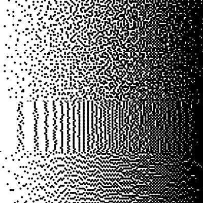

Scanning along horizontal or vertical lines leads to more distinctly visible patterns, compared to the maze and Hilbert curve.
Hill Climbing Optimization
We can treat dithering as an optimization problem. As a general goal, we want the original and the dot-based image to look basically the same after we blur them.
The simplest way to (approximately) solve this optimization problem is to randomly flip some of the pixels and compute whether the new dot-based image is better than the old one. If it is, keep it for the next iteration. If it isn’t, try again. This is a kind of hill climbing, which works quite well when the problem is this simple.
To speed it up, make it more likely to choose points in regions that don’t look like the original image. Also, at the start of the optimization process, flip a large number of pixels. Over time, decrease this substantially. This lets it converge quickly to a rough solution, and then do a better job at the details toward the end.
The following image compares this to other methods. The top two rows use 2D error diffusion along (first row) a maze or Hilbert curve, or (second row) horizontal or vertical lines. The bottom left image uses this optimization, and the bottom right is random comparison.

This is substantially slower than the error diffusion methods that work quite well. But it’s nice to try new things.