If you’re drawing these lines on a computer, there is no need to sort the lines cleverly. However, if you plan to use a machine to draw them, you want to minimize the total time that the machine is moving. If you don’t optimize the line-drawing order, you could spent a lot of extra time watching the pen traveling in the air.
This is very closely related to the Traveling Salesman Problem (TSP), and the simplest solution is a greedy one. Whenever you get to the end of the line that you’re drawing, find the nearest start/endpoint, and start drawing the new line from there. Here’s an example of that, with simple cross-hatching. The travel path is plotted in red.

In this case, the travel distance was reduced from 251% of the drawing distance to 26%. That’s a lot of saved time!
A second greedy approach is to iteratively build a loop. This leads to fewer long jumps but is about half as fast to run. It starts with a pair of lines, and finds the minimum travel distance around the two by reversing the second line, if necessary. From there, pick a random line, and insert it into the loop where it minimizes the travel distance. Repeat until completion.
A third option is to lean on graphs more. Create a minimum spanning tree of the points, then step through the tree (depth-first) to find the order for visiting the points. Discard any repeat visits on this traversal, and it’s a TSP approximation! There are some fancy things to try, such as encouraging the traversal to keep left (or right, as you wish) when stepping from a parent to child node. This makes the path a little less jumpy.
Another option is to use a space-filling curve, like the Hilbert curve used here, to give a spatial index for each point. This is super fast, but introduces some vertical and horizontal artifacts, where you can tell that some grid-based something was done.
The next image compares these different approaches, applied to a bunch of points:
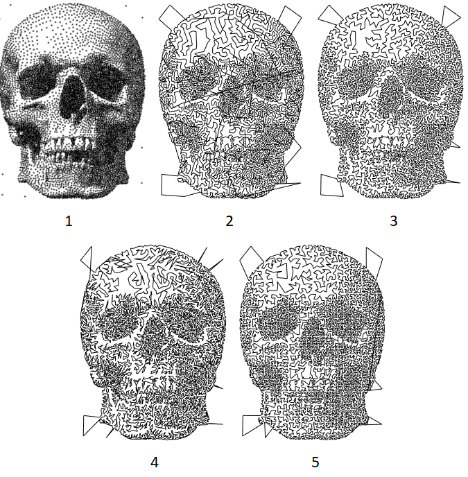
The greedy-loop approach just looks the best. It has few long jumps, it’s not super jagged, and it is pleasantly irregular. With respect to the the travel distance, each of these approaches is basically the same, plus or minus one or two percent.
If you use these algorithms with a large number of points, it’s easy to write versions that are very expensive: scaling quadratically with the number of points. This can be reduced substantially by using a spatial hash, for example.
Application to Halftoning
As you may have noticed from the drawing above, you can use a TSP approach to do halftoning. This has been done a bunch before, but it’s still fun.
What level of darkness do you get for a given point density? Assume that the line width is w, and there are N points in an area A . We can assume that the average distance between points scales as d = c \sqrt{A/N}, where c is a scaling constant. Then we have average darkness in a given area as \overline{K} = N d w/A = c w \sqrt{N/A}. From numerical experiments, c \approx 0.8 .