Modfied Voronoi Diagrams and Stippling

Stippling is pretty neat. Draw a bunch of points and get an image? I like it. This post works up from basic Voronoi diagrams to anisotropic stippling with multiple dot sizes. I’ll stick to 2D for all this, since I like drawing pictures.

Voronoi Diagrams

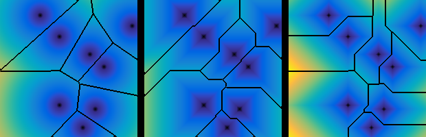
A Voronoi diagram divides up the plane into regions that are closest to a given set of points. And we don’t need to stick to the Euclidean distance, either. For example, the Euclidean distance from point i is \sqrt{ (x-x_i)^2 + (y-y_i)^2 } . The Chebyshev distance is \max \left( |x-x_i|, \, |y-y_i| \right) , and the Manhattan distance is \left( |x-x_i|+|y-y_i|\right) . Look at the resulting diagrams with these different metrics:

Lloyd’s Algorithm

A simple Voronoi diagram just tells you what regions belong to which points. For making uniformly distributed points (AKA a centroidal Voronoi tesselation), Lloyd’s algorithm is great. The basic idea is to repeatedly:

1. Compute the Voronoi diagram
2. Find the geometric center (centroid) of each cell
3. Move each point to the centroid of its cell

And keep doing that until it barely changes. Here’s an animation of that first set of points sliding into place:

That basic approach works well for arranging points uniformly in the plane, but what if we want denser points in some regions? In that case, we include the image’s darkness in an analogue to the center of mass, rather than using the geometric centroid. Simple change, but that leads to effective stippling!

To find define the center of mass, say that the seed point i is at position (p_{x,i},p_{y,i}), its cell region is labeled as C_i, and the image’s brightness is distributed as I(x,y). Then we find the position of the center of mass to be:

\begin{aligned} p_{x,i,new} &= \frac{\int_{C_i} (1-I) \, x \, dC}{\int_{C_i} (1-I) \, dC} \\ p_{y,i,new} &= \frac{\int_{C_i} (1-I) \, y \, dR}{\int_{C_i} (1-I) \, dC} \end{aligned}

When the image is uniform, this is equivalent to computing the centroid.

Multiplicatively Weighted Voronoi Diagram

Let’s mess with the distance functions. For example, the next pair of images uses the Euclidean distance, but the one on the right has scaled the distance from each stipple with random numbers. Each point has some scaling factor, s to have the modified distance s\sqrt{ (x-x_i)^2 + (y-y_i)^2 }

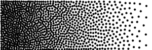
By choosing the proper scaling, we can use this to represent the effect of different sizes of stipples. The solution turns out to be very simple: if the stipple has radius r_i, then s= 1/r_i. Use this in Lloyd’s algorithm, and we get properly spaced stipples of variable size! For example, here’s a circular ramp where the radius of the dots double as you move across the image.

Neat!

Anisotropy

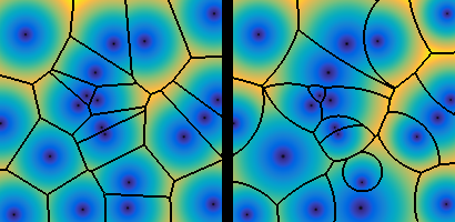
Let’s keep messing with the distance function. If we want the points to be more closesly spaced along a certain direction, we can modify the distance function to use locally transformed axes. Let’s define anisotropy as the ratio between the long axis and the short axis of a scaled shape. Then if we want to have some anisotropy \alpha along an angle \theta , redefine the distance function as:

\begin{aligned} \xi &= (x-x_i) \cos(\theta)-(y-y_i) \sin(\theta) \\ \eta &= (x-x_i) \sin(\theta)+(y-y_i) \cos(\theta) \\ d_i &= r_i ^{-1}\sqrt{ \xi ^2 \alpha + \eta^2/\alpha} \end{aligned}

Here’s an example of \alpha increasing from top to bottom, and \theta varying from left to right.

With anisotropic diagrams, the cells are longer along one axis, so their dots clump up to make apparent lines. This can make some nice effects, sometimes.

Simple implementation

Although there are several efficient algorithms for computing Euclidean Voronoi diagrams, these won’t work well with these modified distance metrics. So I’ll describe my general approach here.

The simplest version first. Define a radius field R(x,y), angle field \theta(x,y), and an anisotropy field \alpha(x,y) over the image area. Randomly place N dots at unique points on the image. For each iteration:

1. Determine the properties of each dot based on its position: R_i, \, \theta_i,\, \alpha_i
2. Calculate the Voronoi diagram using the preferred distance metric, weighted and rotated appropriately for each dot.
3. Calculate the center of mass of each dot’s local region.
4. Move the dot to its region’s center of mass.
5. Repeat until sufficiently converged, or a set number of iterations are performed.

This works eventually, but has a couple problems. Ideally, the total darkness from the drawn dots should be equal to the total darkness of the image. Unfortunately, this is not guaranteed with this approach, but can be fixed by uniformly scaling the dot radii by a factor \rho, which ensures that \rho in \sum_i \pi \left(\rho R_i\right)^2 = \sum\left(1-I\right) .

The second problem is that this approach is terribly slow with a large number of points. There are two ways to speed this up: increase the number of points slowly, and resize the image according to the number of dots. The following algorithm does both those things.

Better implementation

Begin with the initial radius field R_0(x,y), angle field \theta_0(x,y), and anisotropy field \alpha_0(x,y), defined across the initial image I_0 . The initial area of the image is [ latex] A_0 [/latex]. Pick the final number of dots N_f , and place an initial dot anywhere on the image.

1. Choose N_2 , the number of dots to have after this iteration
2. Linearly scale the dimensions of I_0 and R_0 to be proportional to \sqrt{A_0}/N_2 to yield I, \, R.
3. Determine the properties of each dot based on its position: R_i, \, \theta_i,\, \alpha_i.
4. Calculate the Voronoi diagram, using the preferred distance metric, weighted and rotated appropriately.
5. Estimate the number of new dots to have in each dot’s region, then add them:
   1. Calculate the average of R in each region as \bar{R}_i
   2. Calculate the total darkness in each region as D_i
   3. With the scaling c = \sum_i \frac{D_i}{N_2 \pi \bar{R}_i^2} , the new number of dots in each region is approximately N_i = \text{round} \left(\frac{D_i}{c \pi \bar{R}_i^2} \right) . The new total number of dots is N = \sum_i N_i .
   4. Discard the old dots, and randomly distribute the N_i dots in their respective regions.
   5. For a set number of iterations, use the simple version of Lloyd’s algorithm to properly spread those dots within only their region.
6. For a set number of iterations, use the simple version of Lloyd’s algorithm to better spread the dots over the full image.
7. Repeat until N \geq N_f

This has more complications, as well as more knobs to turn. Assuming good convergence, it makes sense to have N_2 \approx 5 N or so. Then the number of iterations within each region can be fairly small, say 5. The number of iterations on the full field can also be small, but it’s worth tweaking. The dimensional scaling works well with about 50 pixels per dot.

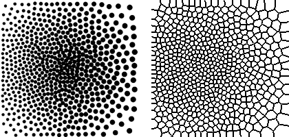
The net result of this algorithm is being able to make complex stippled drawings like this in just a few seconds: